Case Study

The new COE formulation’s contribution to the life-cycle cost analysis is best illustrated using an example. Consider a standard 500-MW CC plant (57.5% rated efficiency) described as Plant A. Two enhancements are planned for Plant A: improved part-load heat rate and a faster start-up and load ramp capability (assumed 50% shorter time). The new product that incorporates these improvements will be called Plant B. The remainder of the key plant parameters and assumptions used in this case study are summarized in Table 1. The beneficial impact of the planned improvements on the COE is conceptually explained in Figure 2.

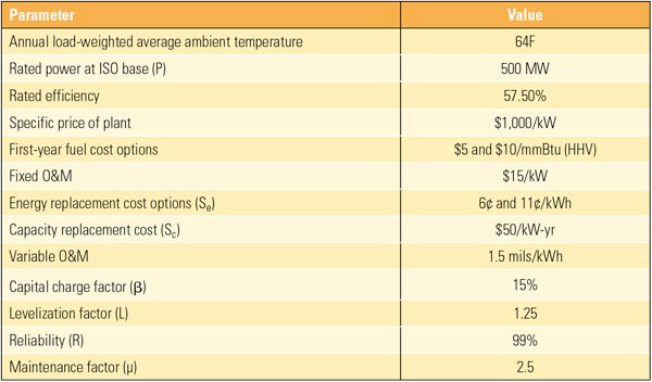
Table 1. Key data and parameters used for calculating COE. The data shown here are for illustration purposes and do not reflect any existing product and/or guarantee. Sources: Electric Power Research Institute, U.S. Energy Information Administration, and PJM

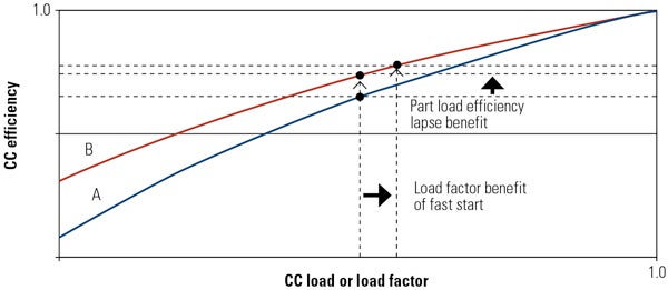
2. Combined-cycle part-load efficiency. Plant B has better part-load efficiency lapse than Plant A in this hypothetical comparison. Thus, at the same average load, B has better efficiency (less fuel consumption) than A. The benefit of the faster start-up capability is a higher effective load factor (less time spent at lower loads) and, consequently, higher efficiency. Note that the generic curves shown here are for illustration purposes and do not reflect any existing product and/or guarantee. Source: GE Energy

3. Calculating the COE. Applying the assumptions listed in Table 1 to the original and modified COE formulas to Plant A illustrates the usefulness of this new way of calculating COE. The assumed price of natural gas used to calculate the COE was $5/mmBtu. An energy replacement cost of $60/MWh was assumed. Values shown in the table are in millions of dollars. Source: GE Energy

Two operating scenarios for Plant B could be analyzed:

• Scenario B1. Plant B reaches baseload quicker than Plant A, allowing the plant to be dispatched for a longer period. Therefore, it generates more revenue—but at the expense of higher total fuel consumption and emissions. H_eff is the same as for Plant A, or 4,552 hours (calculated previously).
• Scenario B2. Plant B starts later than Plant A and reaches baseload at the same time as Plant A normally would. The benefit to operating in this manner is lower fuel consumption and emissions—but at the expense of less generation (less revenue). H_eff is reduced by 150 hours to 4,402 hours.

It would seem that starting a “fast” power plant as early as possible so that it contributes baseload power to the grid quicker (scenario B1) is a better strategy than starting it as late as possible to be online at the last minute (scenario B2). However, this may not be the case when electricity sale prices are taken into account.

If the price before the prescribed time when the market price becomes effective is significantly lower (or even below the variable cost of generation), the apparent advantage of B1 may be much more modest or even nonexistent. In fact, B1 is most likely to occur in an emergency situation, when immediate dispatch is required to exploit an opportunity or to make up for a sudden or imminent loss in generation.

However, B2 is probably the norm for regular plant starts. Furthermore, a plant may have fast-start capability, but the plant owner may choose to use it sparingly or not at all unless paid a premium by a system operator to dispatch on short notice at a significant premium. Thus, the actual value of the fast-start capability is more likely to fall somewhere between the two scenarios. For this example, a weighted average of the performance of the two scenarios is used.

A comparison of the COE calculated using the standard (original) and modified (proposed) formulations is shown in Figure 3. The new formulation returns a 25% higher value, driven by the use of “real” effective kWh and efficiency values (lower than their nominal baseload counterparts) and additional cost components. (Note the significant contribution of emissions even when only CO₂is considered. When NO_x, CO, and other emissions are also thrown into the mix with system-specific “known” costs, the impact will be more pronounced.) The real benefit of the proposed formulation, however, is its ability to account for plant metrics other than rated performance, thereby providing an improved plant life-cycle cost evaluation.

From the equipment supplier’s point of view, an interesting question is now raised: What is the market value of the Plant B upgrades, assuming Plant B COE remains the same as Plant A’s? If the Plant B upgrades are evaluated by assuming 10% unplanned starts (a reasonable assumption given the earlier discussion), then the results, summarized in Table 2, are quite interesting:

• A CC design with a better part-load heat rate has a value of $7 million to $13 million for $5 and $10 fuel, respectively. This is quite significant when you consider that each 0.1 percentage point in rated efficiency is worth ~$1 million to ~$2 million (with the assumptions of this example) for the same fuel price range. The implication is that there is room for about 0.7 net CC efficiency points for a trade-off between ultimate rated performance and sustained performance across a wider load range.
• A nimbler CC design, which slashes the start time and load ramp rate by 50%, has an additional value of $10 million to $13 million for $5 and $10 fuel for a total value of $17 million to $26 million compared with Plant A, assuming no difference in plant reliability, maintainability, or component degradation.
• A reduction of 1% in reliability (R = 98% instead of 99%) is more than enough to wipe out all the value compared with Plant A, or even more (a reduction in value by $15 million to $22 million). The economics worsen if any potentially adverse impact on maintenance factor and/or nonrecoverable degradation is thrown into the mix.
• In order to simplify the treatment herein, NO_x and CO emissions (typically reduced during faster starts) are ignored. Inclusion of either will increase the value of Plant B with the fast-start feature.
• Similarly, in extremely hot climates and/or applications with duct firing, hot day part-load performance characteristics of the plant become important. This refinement can be easily incorporated into the proposed COE formula using applicable correction curves or a load profile table.

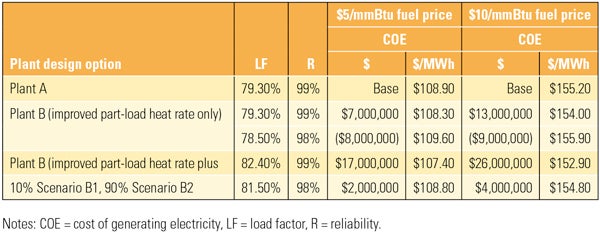
Table 2. Evaluating the COE of two plant design options. Note the dramatic negative economic impact of a small decrease in Plant B’s reliability. The detrimental impact on plant economics would be even more pronounced should a maintenance factor and/or nonrecoverable performance degradation be considered as well. Dollar values reflect the difference from the Plant A baseline. Be aware that electricity sale price or ancillary market opportunities and payments are not included in this analysis. Source: GE Power

The expected increased use of CC plants in the future will place a premium on units that can be heavily cycled and quickly started. By adding these effects to the familiar COE equation, we get a new formulation that can be easily used to perform screening studies to determine the value of a plant more comprehensively.

In most applications, significant life-cycle cost savings are possible for plants that can operate at part load with improved efficiency or that can start and reach baseload faster than conventional plants. Now you have a screening tool to estimate the value of those operational improvements.

For Part 1 of this article please click here.